This article aims to give a broad overview of how neural networks, Fully Convolutional neural networks in specific, are able to learn fluid flow around an obstacle by learning from examples.

This series is divided into three parts.

Part 1: A data-driven approach to CFD (this post)

Part 2: Implementation details

Part 3: Results

Introduction

Solving fluid flow problems using computational fluid dynamics (CFD) can be demanding both in terms of computer hardware and simulation time. Artificial neural networks (ANNs) are universal approximators and are capable of learning nonlinear dependencies between many variables. This article aims to apply artificial neural networks to solve fluid flow problems in order to significantly decreased time-to-solution while preserving much of the accuracy of a full-fledged CFD solution.

An important observation to be made for laminar flow is the fact that the fuid flow at a certain point within the simulation domain is mainly dependent on the flow in its immediate neighborhood, though not heavily dependent on more distant areas in the simulation domain. If the fluid flow in an area changes due to a modified geometry of an obstacle for the fluid, one may expect to see a difference in the immediate neighborhood of this area, but no substantial change to the overall ow behavior in more distant parts of the simulation domain. State-of-the-art numerical solvers do not take advantage of the immediate relationship between small changes in obstacle shape and resulting small changes in flow behavior. They have no “memory” of previous simulations. This work argues that such a memory of previous simulations in combination with learning the connection between simulated geometry and developed fluid flow can be learned by an Artificial Neural Network. Given enough training data for the ANN and a well-suited network architecture, the neural network can be expected to be able to predict flow fields around previously not seen geometries with a hopefully high accuracy. The immense speed in fluid flow estimation once the network was trained gives this data-driven approach to CFD advantages in terms of computation speed under certain conditions.

Creating training data

The neural network should be able to predict fluid flow behavior based merely on the geometry of the object. For the sake of simplicity, this work solely focuses on making the network predict the fluid velocity vectors. Other important field quantities such as density or pressure will not be part of the network training data but may in principle be taken into account as well.

In order to create a training set that is diverse enough in terms of obstacle shapes, obstacle orientation and obstacle size, a way to create geometries of different kinds and shapes had to be found. The shapes had not only to be diverse enough to let the neural network learn the dependencies between different kinds of shapes and their respective surrounding flowfields, but they also had be mesh-able without the need for custom meshing parameters depending on the concrete geometry topology. Due to these constraint, this work focused on creating random two-dimensional polygons. In order to avoid visualization artifacts and to create smooth surfaces, the sharp corners of the obstacle surfaces are smoothed with a laplacian smoothing operation.


Some smoothed polygons used as training data

A critical question to address is how the geometry of the simulation setup can be represented for the neural network. In order to simulate the fluid flow around a specific geometry, it has to be converted into a mesh. This mesh is composed of primitive elements such as tetrahedra or cubes. Slightly modifying the simulated geometry or changing meshing parameters such as element size can substantially change the single element parameters and the total number of elements in the mesh. Fully Convolutional neural networks are designed to only handle input objects of the same size. A straightforward way to map an arbitrary mesh to a regular grid of values is to voxelize it. This is achieved by overlaying the mesh with a regular grid and assigning a value to each of the grid cells depending on the content of the mesh at this point. This process is called voxelization. The grid has the same dimensions for every input geometry and thus allows for one single network architecture for all input geometries while preserving details of the geometry topology.


Fluid velocity in vertical y-direction

Fluid velocity in horizontal x-direction

The simulation data is voxelized in the same fashion. Thus, the simulation data consists of a tensor of shape [height, width, 2] for there are two velocity components to a two-dimensional velocity vector.

The whole work-flow for training-data creation can be summarized as follows:

Geometry generation: Different obstacle geometries with varying shapes are created. They are exported as STL files for later import into a meshing program and also as a numpy array containing the voxel grid of the geometry.
OpenFOAM case setup: This second step creates a geometry-specific OpenFOAM case from a template case and inserts the geometry that was created in step 1.
Meshing: Meshing of the created obstacle geometry.
Simulation: Simulating the concrete OpenFOAM test case. The simulation may reach an end once a convergence criteria is fulfilled. This might be a maximum number of steps or a negligible residuum.
Post-processing: In this step, the OpenFOAM case results are converted into the VTK file format and a pixel/voxel grid of the results is created with paraView and saved to disk.


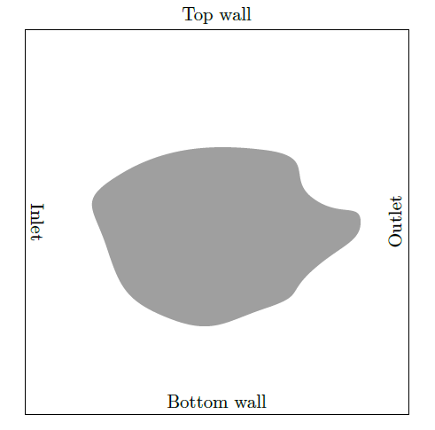
Generic Open-FOAM simulation setup. The fluid streams into the simulation domain through the inlet, goes around the obstacle and leaves the simulation box through the outlet.

Generic Open-FOAM simulation setup. The fluid streams into the simulation domain through the inlet, goes around the obstacle and leaves the simulation box through the outlet.

Network architecture

Fully Convolutional neural networks (FCNs) are widely used for image segmentation tasks where each pixel of the input image is assigned to a class. Each class corresponds to a type of detected object, i.e. car, pedestrian or dog. This property is achieved by first scaling the input image down and applying convolutional and pooling operations just like a Convlutional Neural Network (CNN). However, in contrast to CNNs, afterwards in a second step, the image is scaled up again using so-called deconvolutional operations (also known as transposed convolution) while preserving the assigned labels to each pixel. Deconvolution layers are identical to convolution layers, if the input and output nodes are switched. FCNs are therefore able to take an input of arbitrary shape and assign a numerical value to each of the entries of the input tensor based on the training samples it was given during training.

Thus, a FCN could be able to take a voxel grid of an obstacle, try to predict the fluid flow around the obstacle and compare it with the ground-truth data coming from the OpenFOAM simulation.

The network architecture which was used for this thesis was adapted from (this implementation)[https://github.com/loliverhennigh/Steady-State-Flow-With-Neural-Nets].

The network architecture is kept all convolutional and takes advantage of both residual connections and a U-Network architecture. This proved to drastically improve accuracy while maintaining fast computation speeds. In the context of fluid flow prediction, the task of the network is to assign a floating point number to each pixel of the input tensor, representing the fluid flow velocity at this position.

Since the fluid velocity vector has two components in two dimensions, the FCN outputs two tensors, one for the flow velocity in x-direction and the other one corresponds to the flow velocity in y-direction. Concretely, the output of the neural net is a tensor with dimensions [batchsize, width, height; 2]. The network makes use of several components that have been inspired by PixelCNN++.

Limitations

Laminar fluid flow follows a predictable pattern given a geometry through or around which the fluid flows and a suitable neural network might be able to pick up the complex nonlinear dependencies between simulated geometry and final fluid flow. The structure of fluid flow in reality does not only depend on the shape of obstacles but also on fluid properties such as viscosity, density, and temperature. Other parameters include the type of boundary condition, chemical reactions, and many more. Partially turbulent flows or even fully turbulent flows with higher Reynolds numbers exhibit a much more complex behavior that cannot expected to be modeled by a data-driven approach to CFD.

A physically accurate model of fluid flow accounts for the field quantities flow velocities \(v(x)\), density \(\rho(x)\), pressure \(p(x)\) and inner energy \(e(x)\). In a laminar setup with low flow speeds and no chemical reaction occurring, however,density, pressure, and energy of the fluid are distributed approximately uniformly within the simulation domain and can thus be neglected. Thus, we focused only on fluid flow velocity components in our data-driven approach.

In this work, specific constant fluid parameters and boundary conditions were chosen for the generation of training samples. As a consequence, the learned dependencies between simulated geometry and fluid flow are only valid for a small subset of simulation setups where the simulation parameters are equal or close to the ones used for the creation of the training data set. As these simulation parameters are not encoded into any of the inputs of the neural network in our approach, we do not expect the network to be able to generalize to simulation parameters it was not trained on previously.

Conclusion

We saw that given suitable training data, a Fully Convolutional Neural Network is able to learn laminar fluid flow behavior.

Special thanks to Oliver Hennigh, who made an awesome implementation of a Fully Convolutional Neural Network for fluid flow prediction, which was a huge inspiration for me.