But what exactly are Autoencoders?
In today's post I would like to give you a quick-and-dirty introduction into a neural network architecture type called Autoencoders. The post is aimed at Machine Learning beginners who would like get some basic insights into Autoencoders and why they are so useful.
Concept
Autoencoders are structured to take an input, transform this input into a different representation, an embedding of the input. From this embedding, it aims to reconstruct the original input as precicely as possible. It basically tries to copy the input. The layers of the autoencoder that create this embedding are called the encoder, and the layers that try to reconstruct the embedding into the original input are called decoder. Usually Autoencoders are restricted in ways that allow them to copy only approximately. Because the model is forced to prioritize which aspects of the input should be copied, it often learns useful properties of the data.
More formally, an autoencoder describes a nonlinear mapping of an input \(\mathbf{x}\) into an output \(\tilde{\mathbf{x}}\) using an intermediate representation \(x_{encoded} = f_{encode}(\mathbf{x})\), also called an embedding. The embedding is typically denoted as \(h\) (h for hidden, I suppose). During training, the encoder learns a nonlinear mapping of \(\mathbf{x}\) into \(\mathbf{x}_{encoded}\). The decoder, on the other hand, learns a nonlinear mapping from \(x_{encoded}\) into the original space. The goal of training is to minimize a loss. This loss describes the objective that the autoencoder tries to reach. When our goal is to merely reconstrut the input as accurately as possible, two major types of loss function are typically used: Mean squared error and Kullback-Leibler (KL) divergence.
The mean squared error (MSE) is (as its name already suggests) defined as the mean of the squared difference between our network output and the ground truth. When the encoder output is a grid of values a.k.a. an image, the MSE between output image \(\bar{I}\) and ground truth image \(I\) may be defined as
The notion of KL divergence comes originally from information theory and describes the relative entropy between two probability distributions \(p\) and \(q\). Because the KL divergence is non-negative and measures the difference between two distributions, it is often conceptualized as measuring some sort of distance between these distributions.
The KL divergence has many useful properties, most notably that it is non-negative. The KL divergence is 0 if and only if \(p\) and \(q\) are the same distribution in the case of discrete variables, or equal almost everywhere in the case of continuous variables. It is defined as:
In the context of Machine Learning, minimizing the KL divergence means to make the autoencoder sample its output from a distribution that is similar to the distribution of the input, which is a desirable property of an autoencoder.
Autoencoder Flavors
Autoencoders come in many different flavors. For the purpose of this post, we will only discuss the most important concepts and ideas for autoencoders. Most Autoencoders you might encounter in the wild are undercomplete autoencoders. This means that the condensed representation of the input can hold less information than the input has. If your input has \(N\) dimensions, and some hidden layer of your autoencoder has only \(X < N\) dimensions, your autoencoder is undercomplete. Why would you want to hold less information in the hidden layer than your input might contain? The idea is that restricting the amount of information the encoder can put into the the encoded representation forces it to only focus on the relevant and discriminative information within the input since this allows the decoder to reconstruct the input as best as possible. Undercomplete autoencoder boil the information down into the most essential bits. It is a form of Dimensionality reduction.
Now, let us discuss some flavors of autoencoders that you might encounter "in the wild":
Vanilla Autoencoder
The most basic example of an autoencoder may be defined with an input layer, a hidden layer, and an output layer:
![A simple autoencoder (image credit: [[2]](https://pythonmachinelearning.pro/all-about-autoencoders/))](/images/autoencoder/vanilla.png)
The Input layer typically has the same dimensions as the output layer since we try to reconstruct the content of the input, while the hidden layer has a smaller number of dimensions that input or output layer.
Sparse Autoencoder
However, depending on the purpose of the encoding scheme, it can be useful to add an additional term to the loss function that needs to be satisfied as well.
Sparse autoencoders, as their name suggests, enforce sparsity on the embedding variables. This can be achieved by means of a sparsity penalty \(\Omega(\mathbf{h})\) on the embedding layer \(\mathbf{h}\).
The operator \(\mathcal{L}\) denotes an arbitray distance metric (i.e. MSE or KL-divergence) between input and output. The sparsity penalty may be expressed the \(L_1\)-norm of the hidden layer weights:
with a scaling parameter \(\lambda\). Enforcing sparsity is a form of regularization and can improve the generalization abilities of the autoencoder.
Denoising Autoencoder
As the name suggests, a denoising autoencoder is able to robustly remove noise from images. How can it achieve this property? It finds feature vectors that are somewhat invariant to noise in the input (within a reasonable SNR).
A denoising autoencoder can very easily be constructed by modifying the loss function of a vanilly autoencoder. Instead of calculating the error between the original input \(\mathbf{x}\) and the reconstructed input \(\tilde{\mathbf{x}}\), we calculate the error between the original input and the reconstruction of an input \(\hat{\mathbf{x}}\) that was corrupted by some form of noise. For a MSE loss definition, this can be defined as:
Denoising autoencoders learn undo this corruption rather than simply copying their input.
![Denoised images (Source: [[1]](https://blog.keras.io/building-autoencoders-in-keras.html))](/images/autoencoder/denoised_digits.png)
Contractive Autoencoder
A contrative autoencoder is another subtype of a sparse autoencoder (we impose an additional constraint on the reconstruction loss). For this type of autoencoder, we penalize the weights of the embedding layer by
The operator \(\nabla\) denotes the Nabla-operator, meaning a gradient. Specifically, we penalize large gradients of the hidden layer activations \(h_i\) w.r.t the input \(x\). But what purpose might this constraint have?
Loosely speaking, it lets infinitesimal changes w.r.t. the input \(\mathbf{x}\) not have any influence on the embedding variables. If make small changes to the pixel intensities of the input images, we do not want any changes to the embedding variables. It is encouraged to map a local neighborhood of input points to a smaller local neighborhood of output points.
And what is this useful for, you ask? The goal of the CAE is to learn the manifold structure of the data in the high-dimensional input space. For example, a CAE applied to images should learn tangent vectors that show how the image changes as objects in the image gradually change pose. This property would not be emphasised as much in a standard loss function.
Variational Autoencoder
Variational Autoencoders (VAE) learn a latent variable model for its input data So instead of letting your neural network learn an arbitrary function, you are learning the parameters of a probability distribution modeling your data. If you sample points from this distribution, you can generate new input data samples: a VAE is a "generative model". [1]
In contrast to a "normal" autoencoder, a VAE turns a sample not into one parameter (the embedding representation), but in two parameters \(z_{\mu}\) and \(z_{\sigma}\), that describe the mean and the standard deviation of a latent normal distribution that is assumed to generate the data the VAE is trained on.
The parameters of the model are trained via two loss terms: a reconstruction loss forcing the decoded samples to match the initial inputs (just like in our previous autoencoders), and the KL divergence between the learned latent distribution and the prior distribution, acting as a regularization term.
For a proper introduction into VAEs, see for instance [3].
Experiments
2D-Manifold Embedding
Let us now see how we can embed data in some latent dimensions. In this first experiment, we will strive for something very simple. We first create a super monotonous dataset consisting of many different images of random blocks with different heights and widths, we will call it the block image dataset.
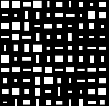
Let us train a VAE with only two latent dimensions on 80000 of these block images and see what happens. I chose to use only two latent dimensions because each image can be visualized by the location of its latent embedding vector in a 2-D plane.
The figure below shows which feature vector in the 2-D plane corresponds to which block image. The block image is drawn at the location where its feature vector lies in the 2-D plane.
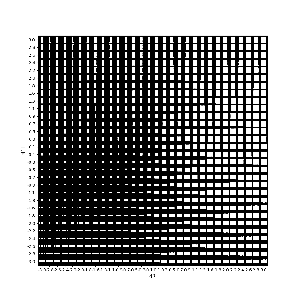
It is quite obvious that the autoencoder was able to find a mapping that makes a lot of sense for our dataset. Recall that each input datum (a single image) has \(height \cdot width \cdot channels = 28 \cdot 28 \cdot 1 = 784\) dimensions. The autoencoder was able to reduce the dimensionality of the input to only two dimensions without losing a whole lot of information since the output is visually almost indistinguishable from the input (apart from some minor artefacts). This astounding reconstruction quality is possible since each input image is so easy to describe and does not contain very much information. Each white block can be described by only two parameters: height and width. Not even the center of each block is parametrized since each block is located exactly in the center of each image.
If you want to play around with this yourself, you can find the code here. Most of the code was taken from the Keras github repository.
Similar image retrieval
While embedding those simple blocks might seem like a nice gimmick, let us now see how well an autoencoder actually performs on a real-world dataset: Fashion MNIST. Our goal here is to find out how descriptive the embedding vectors of the input images are. Autoencoders allow us to compare visual image similarity by comparing the similarity of their respective embeddings or features created by the Autoencoder.
As the Fashion MNIST images are much more information-dense than the block-images from our last mini experiment, we assume that we need more latent variables in order to express the gist of each of the training images. I chose a different autoencoder architecture with 128 latent dimensions.
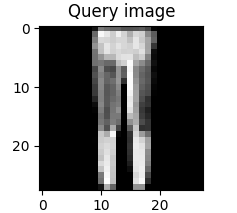
The idea is to to create a feature vector for a query image for which we want similar results from a database. Below we can see an exemplary query image of a (very low-res) pair of jeans.
Using our autoencoder that was trained on the Fashion MNIST dataset, we want to retrieve the images corresponding to the features that are closest to the query image features in the embedding space. But how can we compare the closeness of two vectors? For this kind of task, one typically uses the cosine distance between the vectors as a distance metric.
Here are the four closest neighbors of the query image in feature space:
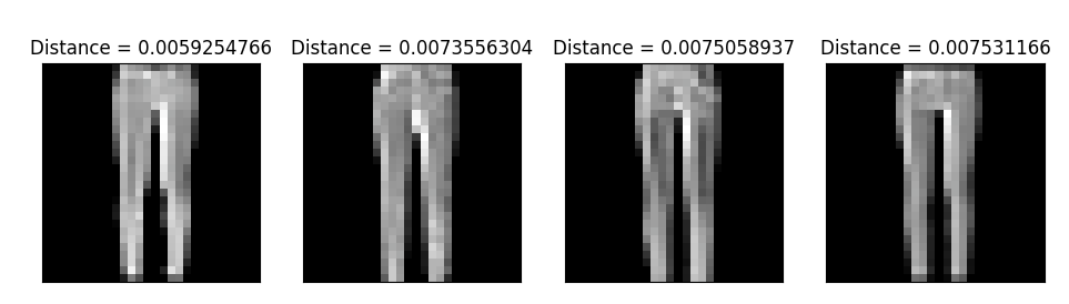
Nice! Pants are similar to pants, I guess!
Lets try again with a new query image:
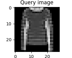
And here are the four closest neighbors:
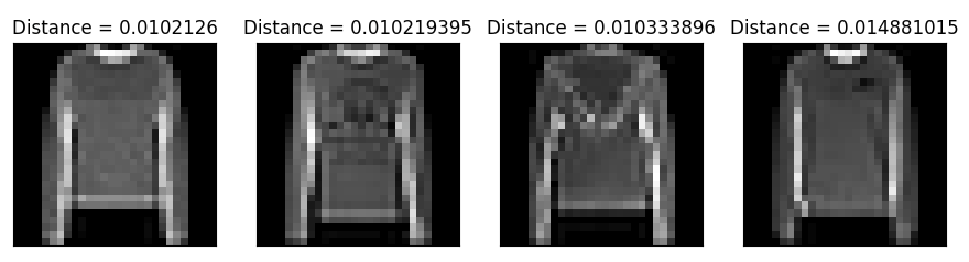
Cool! The autoencoder was definitely able to encode the relevant information of each input image in the embedding layer.
Note: You should bear in mind that the autoencoder was not trained with any labels for the images. It does not "know" that these are images of shirts. In only knows that the abstract features of all of these images are roughly similar and highly descriptive of the actual image content.
If you want to play around with this yourself, the code may be found here.
Conclusion
We have seen how autoencoders can be constructed and what types of autoencoders have been proposed in the last couple of years.
The ability of Autoencoders to encode high-level image content information in a dense, small feature vector makes them very useful for unsupervised pretraining. We can automatically extract highly useful feature vectors from input data completely unsupervised. Later we may use these feature vectors to train an off-the-shelf classifier with these features and observe highly competitive results.
This aspect is especially useful for learning tasks where there is not very much labeled data but very much unlabeled data.
Thanks for reading and happy autoencoding! 👨💻🎉